Background
This unit is divided into three sections, with each section building upon the previous ones. Conventions of set theory and transformations will be used to demonstrate concepts generally, with direct applications to physics given at the end of each section.
Coordinate Systems and Measurement
For the first section, we seek to establish the number line as the foundation of a one-dimensional coordinate system, make measurements within that coordinate system and then geometrically interpret arithmetic operations as measurements along the line.
Coordinate Systems and Their Construction
To do physics in one dimension, we need to start with an appropriate one-dimensional coordinate system. To construct this, we will begin by considering a straight line, which we will call L. To understand the structures of the line and operations on the line, we must consider the important geometric features of L.
The first of the two foundational features is order. Points that lie on the line are ordered, and this ordering it total, meaning that any two points are comparable. For example, if you have two different points p and q, one of them is greater than the other.
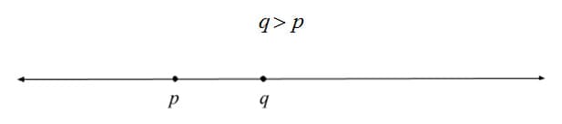
This ordering is also transitive. If another point r is greater than q:

Then its relationship to p is implied:

As a consequence, this also establishes the idea of orientation, or direction, along the line. This orientation corresponds to the sign of numbers, such that numbers greater than 0 are positive and numbers less than 0 are negative. Successively more positive points extend out in the positive direction while successively less positive points extend out in the other, negative, direction.
Order alone is not enough for us to build a viable coordinate system however, because the line itself could to be stretched and squeezed locally while still preserving the order of points. The second feature we need for the line is the inherent notion of distance. Labeled points on the line have a physical separation that can be compared to (and combined with) other separations. On the line, if r is between p and q (that is, p < r < q, or the reverse), and D(p,q) is the distance between p and q, then:
D(p,r) + D(r,q) = D(p,q)
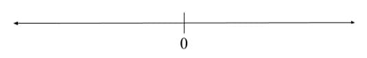
It is the combination of order and distance, along with origin and unit that allows us to coordinatize the line. To do so, we begin from our straight line, L:

To construct a coordinate system on L, that is, to turn L into a number line, we only need to carry out two steps. The first is to choose an origin. This point represents the zero of our coordinate system.
The second is to choose a unit distance, or the distance between 0 and 1.
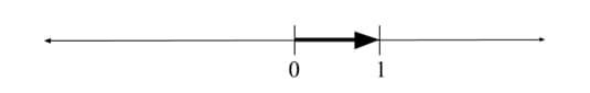
Given these two choices, all other points on the line can be labeled. If you tick off an additional unit distance beyond one, you arrive at the point 2. As you continue adding unit distances, the numbers will be more and more positive. If you travel a unit distance in the opposite direction from zero, you arrive at the point -1.
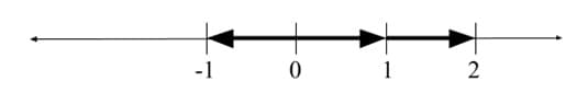
In general, the number labeling any point on the line is the ratio of the distance of that point from 0 to the unit distance, with the sign of the number indicating direction. If that sign is positive, it is in the same direction from 0 as 1. If that sign is negative, it is in the opposite direction.
Every point on the line can be labeled, not just the whole number multiples of the unit distance. All points in between whole numbers can be labeled using rational numbers, decimal expansions or other processes. Regardless of how a point is labeled, the absolute value of the number that labels a point is the ratio of the distance of that point from 0 to the unit distance and the sign of the number indicates the direction from the origin.
Units, Measurement and Precision
If the process of selecting an origin and unit interval seems arbitrary, that is because it is arbitrary. It does not matter where we choose our origin, and it does not matter what the unit distance is, it only matters that the unit distance is established and agreed on in some way. In physics, we have a set of units that we typically like to perform our measurements in, such as meters, kilograms and seconds. That does not mean those are the only viable units, they have just been selected for the sake of convenience and consistency. As long as the unit is specified, measurements can be made using any coordinate system.
The Measurement Principle relates positions on the number line to distances. Formally, the Measurement Principle states: the number labeling a point on the number line tells you the distance of that point from the origin, as a multiple of the unit distance. For example, the point 4 is four times the unit distance from the origin. The Measurement Principle assures that whole numbers are evenly spaced along the number line and dictates where the numbers in between them are placed. Even though the line has order, it is the Measurement Principle that allows us to assign each number to a physical location.
Once constructed, the number line allows us to assign a length to any line-like object. To do so, place the object alongside the number line, with one end lined up with 0. Then the number labeling the point where the other end of the object falls is its length. For example, if the unit distance is 1 cm and a pencil stretches from the origin to the mark labeled 12, that means the pencil has a length of 12 times the unit distance, or 12 cm. While that seems obvious for a ruler, it gives us a clear rule to use to coordinatize the line and an explicit meaning to the numbers that label it.
It is important to have students consider physical limits on precision. When considering a measurement principle, students will naturally connect the number line to a ruler. Even though the number line allows us to label all points using whole numbers, fractions, decimal expansions and rational numbers, a physical tool like a meter stick does not afford the same luxury. If you restrict points on the line to whole number multiples of the unit (or particular labeled fractions), the construction of a physical measuring device puts a hard limit on the precision available when making measurements with it. Specifically, the size of the unit length is going will be a limiting factor. If you take a ruler with a unit length of 1 cm, the measurements that can be made will either be a whole number of centimeters “plus a little more” or “a little less than” a whole number of centimeters. Realistically, that slop at the end of the measurement can be up to half a centimeter. If you refine the unit interval to one millimeter, the maximum size of the “little more” or “little less” is now a tenth of what it was before. Scientists express this as an estimated digit at the end of a measurement.
Measurement Interpretation of Arithmetic
Lengths naturally lend themselves to being combined and compared. This even happens before numbers are defined on the line, because combination and comparison are inherently nonnumeric operations. If you have two pieces of rod, you can put them end-to-end and see the total length. If you would like to see the difference in length between two rods, you can lay them side-by-side and measure the difference. All of this might feels very elementary to students as they do it, but is actually quite subtle and forms the basis for further understanding of the numeric and symbolic representations of arithmetic.
For addition, the picture is easy. Addition is often seen as an operation that combines amounts. Lengths are very simply combined when there is a number line to measure them against. The sum of the lengths is the length of the sum, that is to say the total length of any collection of objects is the sum of the individual lengths. How do we interpret 5 + 7 in this picture? Start from the origin and lay a rod of length five to the right. From the end of that rod, lay an additional rod of length seven. The final sum can be found by measuring the distance from where the rods start to where the rods end and reading off the measurement of the total: 12 units.
Subtraction is slightly more complex. It is frequently viewed as a comparison operation, and it can fill that role. Especially in elementary grades, subtraction can also “take away.” It can also do that. To perform the operation 7 - 5, students may want to take their seven unit rod and their five unit rod and lay them next to each other and see that the difference in size is two units. Along the number line, they would lay the seven unit rod with the left end on the origin and the other end extending to the right. They would then take the five unit rod and line up the right side of it with the right side of the seven unit rod and look at where the left end falls on the number line: two units.
For my juniors, I want them to have the idea that these are merely interpretations of subtraction in a context, not the nature of subtraction in and of itself. Subtraction is, operationally, the addition of the negative. Since positive and negative are defined as specifying direction, we have to care now about how we orient the lengths we combine. To compute 7 - 5, we first consider the addition 7 + (-5). Begin with the left end of the seven unit rod at the origin, allowing the length to extend to the right because it is positive. The five unit rod begins where the seven unit rod ends and the length of it extends to the left, because it is negative. The distance is measured from where the seven unit rod starts to where the five unit rod ends and the result is read off as a position on the number line. Just as above, the result is two units.
Multiplication can be thought of with a similar representation, where 5 x 7 would involve laying five copies of a rod of length seven end-to-end starting from the origin and extending to the right. The result is found by measuring the total length. Division can be similarly represented as the partitioning of a rod, so that 24 ÷ 4 would be breaking a rod of length 24 into four equal pieces and measuring the length of one section. For this unit, however, these representations are significantly less useful than the purposed representation described below of multiplication as a dilation along the line, despite the obvious applications of the measurement interpretation of addition and subtraction.
Vectors and Translations
After students have mastered measurement and the establishment of coordinate systems, it is time to explicitly teach the difference between scalar and vector quantities as well as the representation of arithmetic operations as translations along the line.
Vectors
In physics, we define vectors to be quantities that have a magnitude (or amount), a unit and a
direction. In one dimension, simply specifying whether a number is positive or negative is tantamount
to providing a direction, so the distinction between “number” and “vector quantity”
might not carry a lot of weight for students yet, but many of the major physics quantities, like displacement,
velocity, acceleration, force and momentum are all vectors. Vectors are frequently introduced visually and the
standard picture we use to represent a vector is an arrow. The length of the arrow is the magnitude and the
arrow points in the direction of the quantity that it represents. When referring to vectors symbolically, we
typically put an arrow above the symbol for the quantity to specify that it is a vector and the direction is
something that matters. For example,  }}) would all be symbolic
representations of vector quantities.
would all be symbolic
representations of vector quantities.
Vectors are similar to lengths, in that they are things that naturally want to be added together. This is extremely easy and intuitive to do so using measurement representations of arithmetic. Before, lengths were laid end to end in order to measure the sum. Similarly, vectors are aligned “tip to tail,” meaning that the tip of the first vector touches the tail of the second. It is important to preserve the direction of each individual vector during this process. When performed correctly, the tail of the first vector starts at the origin of your number line and the tip of the final vector in any additive series will live at the sum. Draw a new vector, known as the resultant, from the origin to the tip of the final vector in the additive series. When subtracting two vectors, the direction of the second vector is reversed and the addition process is followed. Remember that subtraction is the addition of the negative and realize that reversing the direction of a vector creates its negative. In one dimension, students should be able to grasp this relatively quickly, since it is relatable to the measurement interpretation of addition, only rods have been replaced with arrows. The figure below demonstrates what is often called the “parallelogram rule for addition.” Seeing that the order in which we combine vectors A and B does not matter, we demonstrate the commutativity of vector addition.

Transformational Interpretation of Arithmetic
Where this unit begins to diverge from conventional presentations in a physics classroom is in the interpretation of arithmetic operations as transformations along the number line. The usual geometric picture of vector addition implicitly assumes that we can translate a vector without changing its length or direction, which allows us to create the standard visual associated with adding vectors. Translating one of the vectors by the other creates the sum. Since vectors in an introductory physics course represent quantities that are associated with motion, the connection is meant to appear naturally. Let us consider first the result of translating an arbitrary point x by a, written Ta(x). What Ta will do is shift all points on the number line by a units. If a is positive, it will shift to the right, and if a is negative, it will shift to the left.
Ta(x) = x + a
This illustrates how the translation Ta, takes any point xand moves it to the new position x + a. Since all points on the number line are shifted by the same amount, we see that translation preserves the distance between two points. Transformations that preserve distance are known as isometries. Isometries also preserve signed distance, or a distance that also specifies a positive or negative direction. On the line, this is the same as vector difference. To demonstrate this, let us apply Ta and observe the signed distance between the points p and q before and after. Before transformation, we find the signed distance, D⃗, through subtraction.
D ⃗(p ,q ) = q - p
Apply the transformation to both points.
Ta(p) = p + a
Ta(q) = q + a
Now we will calculate the new signed distance to see that agrees with the previous result.
D ⃗(p + a, q + a) = (q + a) - p + a)
Apply the associative rule:
D ⃗(p + a, q + a) = q + (a – (p + a))
By the sum rule for inverses:
D ⃗(p + a, q + a) = q + (a + ((- p )+ (- a)))
By the commutative rule:
D ⃗(p + a, q + a) = q + (a + ((- a )+ (- p)))
By the associative rule:
D ⃗(p + a, q + a) = q + ((a + (- a))+ (- p))
Apply the definition of inverse:
D ⃗(p + a, q + a) = q + (0 + (- p ))
Apply the identity rule:
D ⃗(p + a, q + a) = q + (- p )
Finally use the definition of subtraction:
D ⃗(p + a, q + a) = q - p
What does a translation do, then? It adds a fixed quantity to each and every point on the number line, mapping it to a new point. Because distance and scale are preserved, translations are isometries: they do not alter the units of a quantity. With vectors, a displacement vector takes the position of an object and maps it to a new position. A displacement behaves like a transformation, in the sense that each represents a change. The difference is that displacements are a change in position of a particular point, while transformations are a change in the entire line: every point is being displaced in the same way at the same time.
The second type of transformation to consider is dilation. A dilation, dm, will take every point on the line and multiply it by the constant factor m. Symbolically, this is written as
dm(x) = mx
Dilation is not an isometry. To demonstrate why this is the case, let us again look at the distance between points p and q before and after the dilation.
dm(p) = mp
dm(q) = mq
Calculate the distance between the new points.
D(mp,mq) = mq – mp = m(q – p)
Notice now that the new distance between them is m times the old distance. Dilation stretches all intervals on the line by a factor of m. Because it does not preserve distance, dilation results in a change of units. The distance between zero and one is no longer the same as it was. It is scaled by a factor of m.
This is precisely what occurs during the multiplication of a vector quantity by a scalar quantity. Scalars are quantities that have numbers and units, but no direction. Multiplying a vector by a scalar transforms it to a new number line with different units, distorting its length in the process. Dilation of the line is the same thing as a rescaling of the line.
Applications to One Dimensional Kinematics
The purpose of considering addition of vectors and multiplication by scalars as transformations of the number line is to add an additional level of visual and spatial understanding to students’ understanding of the way quantities combine in physics. To illustrate the idea, first consider displacement.
Dx⃗ = x⃗ - x⃗0
x⃗ =x⃗0 +Dx⃗
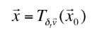
An object’s displacement is equal to its change in position, or, stated differently; an object’s final position is equal to its initial position plus its displacement. When we look at the physical operation performed by displacement, we can view it as a translation of the object byDx⃗. Adding the displacement vector to an object’s position translates the object’s position byDx⃗ and leaves the unit untouched. To use the notation of transformations, we can write:
x⃗ = TD x⃗(x⃗0)
Now consider the displacement undergone by an object moving with a constant velocity over some time interval.
Dx⃗ = v ⃗t
While we say vectors want to be added, for this to work they must refer to the same unit. Positions and displacements, typically, are measured in meters while velocities, typically are measured in meters per second. These are incompatible! Velocities can never be added to displacements. What multiplication by the scalar quantity t does, however, is dilate the velocity vector onto a number line where the fundamental unit is the same as that of displacement, allowing it to be treated as a translation of the position vector.
Dx⃗ = dt v⃗
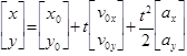
To develop this idea this even further, consider the position equation for a particle undergoing constant acceleration.
Students might be tempted to draw a picture of the particle in the problem, label the velocity and acceleration vectors and then somehow combine them. If they instead view this as two successive translations, first by v⃗t and then by 1/2 a⃗t2 , they can see that while both terms of the equation carry separate physical meaning, but they still translate the position of the particle. Then each piece of the translation can be described by a vector. Even though each piece is based around a velocity or acceleration, they have been dilated by an appropriate factor of time, producing units of a displacement vector. Attending closely to this issue of units separates vectors with incompatible units and reminds students to only add vectors that are expressed in the same unit. Following that line of logic, the standard kinematics equation could then be restated in the notation of transformations as:
The notation is obviously extremely cumbersome, but highlights an essential insight about vectors. Viewing the vectors as transformations emphasizes the impact of physical quantities on each other and provides an intuitive framework by which they can interact.
Two Dimensional Extensions
We have seen how the number line effectively constitutes a coordinate system on the line, provides the framework for measurement and grounds our visual representations of vector addition. The language of transformations provides another way to consider vector addition and scalar multiplication that works with our understanding of the number line, not against it. Fortunately for the world (and somewhat unfortunately for our students) physics is applicable in more than one dimension and these concepts can be extended to provide an intuitive two-dimensional treatment of vectors.
Construction of Two Dimensional Coordinate Systems
When we want to examine motion in the plane, a one-dimensional coordinate system as previously constructed will no longer suffice. That does not mean we ought to disregard our prior work. Indeed as gradually realized during The Middle Ages and finally crystallized by Descartes, we can describe the plane using two number lines.
To construct the plane, we begin by choosing a point for the origin.

Next, we choose an oriented line going through the point for the x-axis.

Next, we select a unit distance on the x-axis to set the scale.

Next we construct a second line, perpendicular to the first one at its origin. On this, the y-axis, we orient another unit distance that is the same length as the first. This sets both axes to the same scale while simultaneously orienting the y-axis.
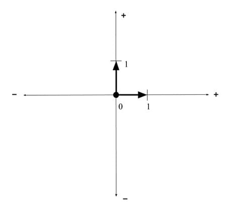
Each line, or axis, retains all of the properties of the original line, such as order and directionality and distance, but we can now describe the position of a point anywhere in the plane, even if it does not lie precisely on one of our axes. The usual convention is to refer to these axes as x and y, with x being associated with the horizontal direction and y being associated with the vertical direction, though other orientations can be equally valid.
The most common way we locate a point in the plane is using Cartesian coordinates. This is a pair of numbers, (x,y), such that when perpendicular lines are drawn from the specified point to each axis, these lines intersect the axes at the values x and y.
A less common way of describing position in the plane is that of polar coordinates, where a number line is “tacked” at the origin but free to rotate and points are specified based on their distance from the origin and the orientation of the line used to measure them. These coordinates are reported in the form (r,Ɵ), with r being their distance from the origin and Ɵ being an angle that describes the orientation of the line of measurement. For standard coordinate systems, the angle Ɵ = 0 describes a line of measurement that points directly along the x axis and the positive direction for Ɵ is defined to be counterclockwise from there. Polar representations better display magnitude and direction but Cartesian representations support vector addition. The big issue is that polar coordinates are wedded to the point around which they are defined, and do not support simple descriptions of translation the way Cartesian representations of components do. To switch between representations, one only needs to know a small amount of trigonometry to derive the following relations:

For students, this can all be derived using only the sine, cosine and tangent relationships as well as the Pythagorean Theorem. In practice, this typically warrants an early crash course in trigonometry for the benefit of those who have not taken a course in it yet and periodic refreshers throughout the year.
Measurement and Vector Notation in Two Dimensions
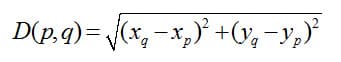
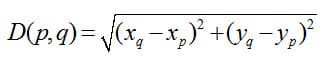
Measuring the distance between two points in a plane can be accomplished by using the Pythagorean theorem. Starting with two arbitrary points p and q, we label the coordinates of these points (xp,yq) and (xq,yp) respectively. Placing them on the plane allows us to visualize the distance between the points, D, as the hypotenuse of a right triangle formed with p and q as the acute vertices.

To find D we write the relationship between the side lengths of this triangle using the Pythagorean theorem:
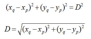
Solving for D gives us a generalized two-dimensional distance formula. Moving forward, we express the distance between two points p and q as D(p,q) such that:
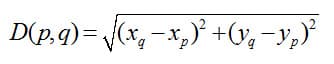
As in one dimension, the distance between two points p and q is the magnitude of the vector drawn from p and q. Unlike in one dimension, merely specifying a positive or negative number is no longer sufficient to fully define that vector in two dimensions. The mention of polar descriptions of points comes from the fact that, especially in applied physics, quantities are most often reported as an overall measurement in a particular direction. The entire notion of measurement in the polar system arises from the ability to align your number line in the direction you want to measure, report how long it is and then specify how you were holding your ruler when you made the measurement. This is intuitive and easy until you need to combine or transform measurements. The danger is that lengths can be combined in any orientation, but the treatment of that is more complex if they are not pointing in the same direction. To get around this, physics typically deals with the components of vectors, which are the perpendicular pieces that lie along a fixed pair of axes and combine to form a vector.
There are three common notations used at this level, each with benefits and drawbacks. The most common, and simplest, is known as ordered set notation. Consider a vector that points from the origin to a point (x,y) in the plane. This vector would also have some length, r, and some direction, Ɵ as found from the relations above. In ordered set notation, we can report this vector as <r,Ɵ>. We can also specify the same vector by referencing its components along the axes, x and y. These can be again computed using the same relations we used above, so the vector can also be represented in ordered set notation as <x,y>. The usage of pointy brackets differentiates the point from the vector directed from the origin to that point. The benefit of using this notation is that it is extremely simple. The downside is that students can lose sight of the difference between a point in the plane and a vector starting at the origin directed toward a point in the plane.
A second representation, known as unit vector notation, is extremely common in college-level physics. We start by specifying a pair of unit vectors, î and ĵ. These are vectors with a length of one unit directed in the positive x and y directions respectively. Placing î and ĵ on the plane appears as so:

Vectors are then represented as a sum of the magnitude of each component multiplied by the appropriate unit vector. So the vector we represented above can be expressed as:
<x,y> = xî + yĵ
A pleasant feature of this notation is that it is an explicit extension of the previously stated Measurement Principle. The unit vectors î and ĵ are the symbolic expressions of the unit lengths and directions we specified back when we originally constructed number lines and this notation shows the total vector as a combination of multiples of these unit lengths. The downside is that the overall length, r, is not immediately apparent, nor is the angle defining the direction easy to read off.
The final notation to consider is known as column vector notation. This is commonly used when matrix operators are introduced, and it will also be the notation of choice for this unit moving forward. The column vector notation is shown with the coordinates arranged in a 2x1 matrix as such:

The unit vectors, î and ĵ, are column vectors of the form:

The unit vector and column vector notations can be connected by replacing î and ĵ with their column vector representations.
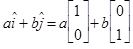
The unit vectors can then be scaled by their magnitudes, a and b:

Combine components in the same directions:
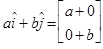
Recover the expected expression, realizing that the column vector is the sum of scaled versions of î and ĵ.

The value of using column vector notation is that it makes obvious later on that physics in multiple dimensions is done using systems of vector equations linked by scalar parameters. Whatever the representation that is chosen, it is important to instill in students that while vectors may be reported as magnitudes and directions, vector addition is performed in terms of components. It is also worth noting that as you progress to higher dimensional spaces in column vector notation, components stay tidy while polar analogs get more and more challenging to work with.
Transformations in Two Dimensions
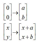
Let us now examine how translations work in the plane. Starting with a translation that shifts all points in on the line in the positive x direction by a units, we wrote:
Ta(x) = x + a
That was fine for one dimension, but now we have two to consider. Just as we needed to represent vectors differently, we must represent translations differently. To extend the previous example to two dimensions we write a translation that shifts all points in the plane in the positive x direction by a units.
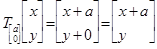
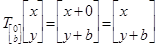
Notice that the quantity being translated and the amount it is being translated by are of the same form. Since translations are additions, performing translations (just as combining quantities) requires the same unit. Vectors translate vectors. Now let us consider a translation of all points in the plane by b units in the positive y direction.
To combine the two translations, we must first understand the composition of transformations. Consider two arbitrary transformations, J and K. The composition of J and K takes an arbitrary point x and transforms it first according to K and then the result of that transformation is transformed according to J.
(J°K)(x) = J(K(x))
Now compose two successive translations, first by b units in the y direction and then by a units in the x direction.
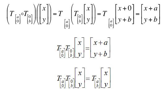
Notice that this applying them sequentially provides precisely the result we would expect by applying them simultaneously. Translations performed along one axis do not affect the coordinate along the other axis. A two-dimensional translation is the composition of two one-dimensional translations along different axes.
Does a two-dimensional translation preserve the distance between two points? Realize first what happens to the origin and endpoints of the vector in the previous example.
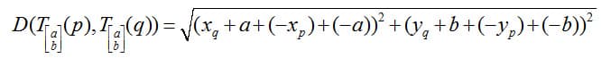
To verify that distance is preserved under two-dimensional translation, we will use the distance formula defined above. Start by remembering the distance between two points p and q is:
Now let us apply an arbitrary two-dimensional translation,  , to these points:

Finding the distance between the transformed points:

By the associative rule and the sum rule for inverses:
By the commutative rule:

By the associative rule:

By the definition of inverse:

Apply the identity rule and the definition of subtraction:

Providing precisely the same result from above! It is also important to note that, when considering the triangles we drew above, the length of the horizontal and vertical sides also remains unchanged. So we can say that for an arbitrary two-dimensional translation, the distance between any two points is preserved:

Since vectors are drawn between points, the length of the translated vector will remain unchanged, meaning that two-dimensional translations are also isometries. Because the distance between the points and the horizontal and vertical separations between the points remain unchanged, the angles in the right triangles we use to determine the distance must also remain the same because of triangle congruence. Thus, we demonstrate that two-dimensional translations also preserves the direction of vectors.
Now consider dilations. We know from one-dimensional situations that multiplication by a scalar dilates a vector. Dilation by a scalar quantity m stretches the vector by a length m.
dm(r) = mr
To determine the effect on the components of that vector, realize that from the relationships above, components have a linear dependence on the length of the entire vector. That is to say, if r doubles, each of the components will also double. Dilation and, by extension, scalar multiplication, multiply each component of a vector by a fixed value.

We can check that dilation is a similarity, or that it stretches all distances by the same factor, using the distance formula. Since vectors are drawn between points, we will investigate the effect of a dilation on two arbitrary points. We found previously the distance between arbitrary points p and q to be:
What about the distance between dm(p) and dm(q)? First, let us apply the dilation to p and q to get the coordinates of the transformed points:
dm(p) = (mxp,myp)
dm(q) = (mxq,myq)
Using the distance formula:

Factor using the distributive rule:

By the distributive rule for exponents:

Factor again using the distributive rule:

Bring the m outside radical by taking the square root:

Demonstrating that the dilation by m stretches all distances by the factor m:

It is important to note that while dilations do not preserve length, they do preserve direction up to sign. The vector will be stretched, but can only end up pointing in precisely the same direction as it did originally (if m is positive) or in the exact opposite direction (if m is negative).
In two dimensions, there exists another transformation that can be used to produce a change of coordinates: the rotation. In an introductory high school physics course, rotations are only treated in special cases. Rotations can be expressed by a rotation matrix, RƟ, as shown:
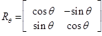
Column vector notation becomes especially helpful here, because it allows for rotations to be computed using matrix multiplication:

In practice for the introductory physics student, however, situations can be simplified by dealing with the situation in a polar representation, where the angles will merely add. As an example, for a point p expressed in polar coordinates:
p = (r,Ɵ)
For a rotation by an angle φ, Rφ, its effect on point p can be expressed as:
Rφ(p) = (r, Ɵ+ φ)
Applications to Physics in Two Dimensions
Column vector notation is especially helpful in illustrating that introductory physics in two dimensions is just the artful combination of two one-dimensional cases. To describe an object moving in the plane under constant acceleration, a typical text might have students set up a system of two parametric equations for the x and y directions.

A more intuitive and informative expression links these components into their original vectors and unites the common scalar parameters.
Based on our previous one-dimensional example, we can see that there are two dilations in the equation that rescale the velocity and acceleration vectors into displacements. These dilations do not let the velocity and acceleration remain on their original planes, but instead take a velocity plane to the displacement plane and an acceleration plane to the displacement plane so they may later be combined.

And these displacements translate the original position into the final position.

Notice that the total effect on the position is two successive translations. When we look at the composition of two successive translations, the result is a single translation by the sum of their individual shifts. In physics, we refer to the idea that the total change on a system is the sum of the changes as the superposition principle. The interesting insight is that viewing vector addition through this transformational lens makes the superposition principle appear as a natural consequence. Because the translations commute, we are mathematically justified in applying them in any order we see fit and the total translation is the sum of the individual translations. The usefulness of the approach does not stop here. Beyond kinematics, momentum is the dilation of velocity by mass.


Similarly, Newton’s Second Law says that force is the dilation of acceleration by mass:


The picture of vectors and physics as transformations lends an inherent physicality to the process of vector addition and scalar multiplication while portraying equations as the series of physical dilations and translations they represent. It also provides students who have not yet learned calculus the opportunity to take notice of the relationships between quantities and how they vary.
Comments: