Big Numbers, Small Numbers

Counting

Counting allows us to enumerate all possible outcomes resulting from events. An event is a particular situation, experiment, or process with a finite set of potential outcomes. Familiar examples are the throw of one or more dice, or the flipping of a coin. There are various methods to assist one when enumerating all elements of an event: methods introduced throughout grade school include making lists, keeping a tally, drawing a tree diagram, or computations using formulas.

At the high school pre-calculus course level, students are expected to enumerate the total number of possibilities for a variety of events. In both Integrated Math II and Math Analysis, the content covered begins with what is called the Fundamental Counting Principle, defined below. The Fundamental Counting Principle is also known as the Multiplication Principle in Combinatorics (8). However, this unit begins with the Addition Principle, defined below, that is not emphasized in high school, but is subtly implied in most situations.

Addition Principle

The addition principle defines a way to break down one event into two, or more, smaller events. These smaller events can be described as subevents of a single event.

Addition Principle: Suppose there are n₁ outcomes (ways) for the event E₁ to occur and n₂ outcomes (ways) for the event E₂ to occur. If all these ways are distinct, then the number of ways for E₁ or E₂ to occur is n₁ + n₂.

Example #1: Addition Principle

A class consists of 16 sophomores and 14 juniors. You will pick a student in the class for a prize. How many ways are there?

Solution: Let E=number of ways to pick a student. To find the number of ways, we must count how many students are in the class. Since there are 16 sophomore and 14 juniors, then E = 16 + 14 = 30 ways you can pick a student to win the prize.

Problem contexts designed for schools often state how many ways an event can occur. However, the addition principle is a key step that my students do not take into account. To compute probabilities, often my students struggle with adding up the number of ways to achieve successes or failures. Emphasizing the Addition Principle will help prepare my students for

Multiplication Principle (Fundamental Counting Principle)

Multiplication Principle: Suppose that an event E can be split into two events E₁ and E₂ in ordered stages. If there are n₁ ways for  to occur, and if for each of these, there are exactly n₂ ways for  E₂ to occur, then the number of ways for the event E to occur is n₁ ∙ n₂. For each outcome of  E_1, there are n₂ possible outcomes for  E₂.

Example #2: Multiplication Principle

You are picking what to wear to school. You have 6 shirts and 4 pairs of pants. How many outfits can you make? To find the number of outfits, we can break the situation down to two events. E₁ represents the number of shirts and E₂ represents the number of pants. Then E₁ = 6 and E₂ = 4. To find the total number of outfits, we multiply the number of ways each event can occur, giving us the image: .

In this example, the events are independent, where the outcome of the first event does not affect the number of outcomes in the second event. Sometimes events are not independent, but still there are the same number of possibilities for E₂, for any outcome of E₁. The multiplication principle is a special case of the addition principle, when every outcome of E₁ leaves the same number of possible outcomes for E₂.

Generalized Multiplication Principle

The multiplication principle can be applied to situations where there are more than 2 events. This fact is buried in the margins of our textbook as a side remark regarding the generalization of the formula. During this unit, I will introduce my students to the Fundamental Counting Principle as it is stated above, and I will also formally generalize the principle to include more than 2 events.

Multiplication Principle (General): Suppose that an event E can be described as, a combination of events E₁, E₂, …, E_k that occur in successive stages. If there are n₁ ways for E₁ to occur, n₂ ways for E₂ to occur for any outcome of E₁, …, and n_k ways for E_k to occur for any outcomes of the earlier events, then the number of ways for the event E to occur is given by n₁ ∙ n₂… ∙ n_k.

Example #3: Multiplication Principle – More than 2 Events

In the state of California, each standard automobile license plate number consists of a one-digit number followed by three letters followed by a three more digits. Digits and letters can be repeated. How many distinct license plate numbers can be formed in California?

Solution: Break up 1 license plate into 7 independent sub events. Each event is either a digit from 0-9 or a letter from A-Z.

Thus there are (10)∙(26)∙(26)∙(26)∙(10∙10∙10)=175,760,000 possible license plate combinations in California.

When I taught this topic in previous years, some of my students would think that this number is very large and therefore incorrect. To build their number sense, I would have students compare the above result with the fact that at the end of 2017 the California DMV reported that there were 25,467,663 registered cars in the state (3). Also, approximately 2.1 million cars were sold and registered in California during 2016. Suppose that rate stays the same and license plates with the standard pattern described above are still issued. If the next license plate to be issued is 8FAA000, and the digits are increased by 1 such that the next plates issued are 8FAA001, 8FAA002, 8FAA003, and so on. This continues to 8FAA998, 8FAA999, 8FAB000, and 8FAB001. This pattern continues until the last license plate 9ZZZ999 is issued. About how long will it be before California issues all possible combinations? If there were 4 digits and 3 letters, but a letter could occupy any position, how would that change the number of possible license plates?

A related question involves the California driver’s license which consists of 1 letter followed by 7 digits. How many different licenses can be issued? When will California need to change the configuration for driver’s licenses?

Permutations

A permutation is a way in which a set or collection of things can be ordered or arranged. The number of permutations of n elements is n∙(n-1)∙3∙2∙1=n!, where the possibilities at each step depend on previous choice, however the number of items does not. I will emphasize how factorial, !, is a mathematical convention that follows directly from the Fundamental Counting Principle. I will present my students with situations where utilizing the factorial notation would allow for computations to be written concisely. I will also compare factorials as analogous to exponential notation for powers of a fixed number.

Example #4: Permutations

Place students into groups of varying sizes and have them determine how many ways they can rearrange themselves in a line. Record the different ways they can line up.

For my classes, I will assign students into groups of different sizes. When placed into groups of 1 student, 2 students, 3 students, and 4 students, I would have each group physically line themselves up into as many different permutations and then record each of the different permutations. 

Group of 1: Since n=1, and 1!=1 There is only 1 way that a student can line up.

Group of 2: Since n=2, and 2!=1∙2=2. There are 2 ways that students can line up.  

Group of 3: Since n=3, and 3!=1∙2∙3=6. For 3 students, they can arrange themselves 6 ways.

Group of 4: Since n=4, and 4!=1∙2∙3∙4=24. With 4 students, they can arrange themselves 24 ways.

I would consider using a group of 5 students, but since that there are 5!=120 different ways students can line up. I would have the students write out all of the permutations, but would not expect them to arrange themselves into each of the ways.

Combinations of n Elements Taken r at a Time

When given a set of n elements, we can count the number of permutations when ordering all n elements. We can also find the number of permutations when ordering less than all of the elements. When choosing r elements from the total set of n, where r<n, the number of permutations for the r elements is given by the formula ^⧠_nP^⧠_r = n!/(n-r)!. The notation ^⧠_nP^⧠_r represents the number of permutations when taking a subset of r elements taken from a set of n elements. The formula and notation is used in the Integrated Math II and Math Analysis textbooks.

My students like to have a formula and will substitute the first numbers they see in a given problem. If I were to follow the lesson as prescribed, my students would only need to identify the values for n and r, substitute into the formula, and compute. I plan to show the connection between the Fundamental Counting Principle and the formula for ^⧠_nP_r through examples.

Example #5: Permutations, nPr

Suppose there are 8 runners in a race. How many ways can they finish 1^st, 2^nd and 3^rd?

Solution: Let E represent the total number of outcomes. The event can be broken down into three smaller components. Let E₁ be the number of ways anyone in the race can finish 1^st, E₂ be the number of ways anyone remaining in the race can finish 2^nd, and E₃ be the number of ways the remaining runners can finish 3^rd.

Then,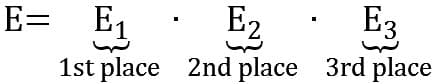

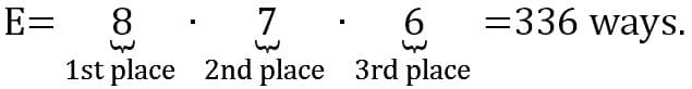
Since there are 8 runners, there are 8 different outcomes for 1^st place, thus E₁ = 8. For second place, there are only 7 runners remaining, giving E₂ = 7. Finally, there are only 6 runners left for third place, giving E₃ = 6. The total number of permutations is

Using the preceding approach shows that the problem can be solved using the Multiplication Principle. ^⧠_nP^⧠_r can be represented as a product of integers from n to (n-r-1). Thus, ^⧠_nP^⧠_r = n!/(n-r)! = n(n-1)(n-2)∙∙∙(n-r-1). This representation is not presented in the Integrated Math II and Math Analysis textbooks. I plan to discuss with my students how this generalized representation really is the Multiplication Principle when we have the number of outcomes is decreasing by one each time.

Solution using Formula: In this scenario n=8 and r=3. Substituting into the formula for ^⧠_nP_r,we have ^⧠_nP_r = 8!/(8-3)! = 8!/5! = (8∙7∙6∙5∙4∙3∙2∙1)/(5∙4∙3∙2∙1) = 8∙7∙6 = 336.

Understanding the problem in context can help better understand why we divide. The first observation would be (n-r) is the number of runners that do not finish first, second, or third. By taking (n-r)!, we are finding all the permutations for the remaining five runners to finish in 4^th, 5^th, 6^th, 7^th, and 8^th place. Since we are only interested in finding the number of ways for the top three finishers, we would divide the total number of race outcomes, 8!, by the number of ways in which the 4^th through 8^th place runners would finish, 5!. The result gives us the same value as using only the Multiplication Principle.

Deriving the Formula

I will show my students that the formula in the textbook can be derived from the product identified in the first solution. Starting with ^⧠_nP^⧠_r = n!/(n-r)! = n(n-1)(n-2)∙∙∙(n-r-1), I will continue the product one step at a time from (n-r) down to 1, and simultaneously dividing from (n-r) down to 1. I will show the following steps:

^⧠_nP^⧠_r = n(n-1)(n-2)∙∙∙(n-r-1) =

= n(n-1)(n-2)∙∙∙(n-r-1)(n-r)/(n-r) =

= n(n-1)(n-2)∙∙∙(n-r-1)(n-r)(n-(r-1))/(n-r)(n-(r-1)) =

...

= n(n-1)(n-2)∙∙∙(n-r-1)(n-r)(n-(r-1))∙∙∙2/(n-r)(n-(r-1))∙∙∙2 =

= n(n-1)(n-2)∙∙∙(n-r-1)(n-r)(n-(r-1))∙∙∙2∙1/(n-r)(n-(r-1))∙∙∙2∙1 =

= n!/(n-r)!.

The result from the Fundamental Counting Principle now coincides with the factorial notation formula found in the textbook. With my classes, I will compare the amount of work it takes to use the textbook formula to perform the computations to arrive at the same answer that can be found through a few multiplications. I often hear my students ask for a formula because many like the fact that you can plug in numbers and compute a result. I want my students to recognize a formula may appear compact and easier, but alternative approaches may be more efficient for actually doing computations.

Combinations

A combination is a subset of a larger set in which the order of elements is not important. The equation for combinations is given and students are tasked with computing the number of combinations by identifying the total number of elements, n, and the number of elements being selected, r.

^⧠_nC^⧠_r = n!/(r!∙(n-r)!) = ^⧠_nP^⧠_r/r!

Why do we divide the number of permutations ^⧠_nP^⧠_r by r! when finding the number of combinations? Just as for the formulas for permutation, the text gives no explanation regarding what is happening with this equation. We will provide an explanation below, after discussing some examples.

Example #7: Lottery

To play the California Fantasy Five lottery game, a person picks five numbers from 1 to 39.  They need to match all five of the numbers. Find the total number of all 5-number combinations.

I would introduce this problem prior to giving the ^⧠_nC^⧠_r. To come up with the solution, I would show how to begin solving the problem by thinking of it as another permutation problem.

Solution: Let E represent the number of ways to select five numbers. To find the number of permutations for the number of ways to select five numbers, the event can be broken down into five smaller events.

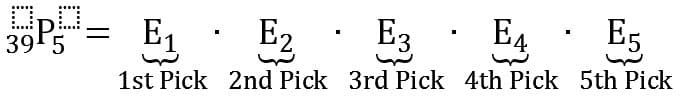
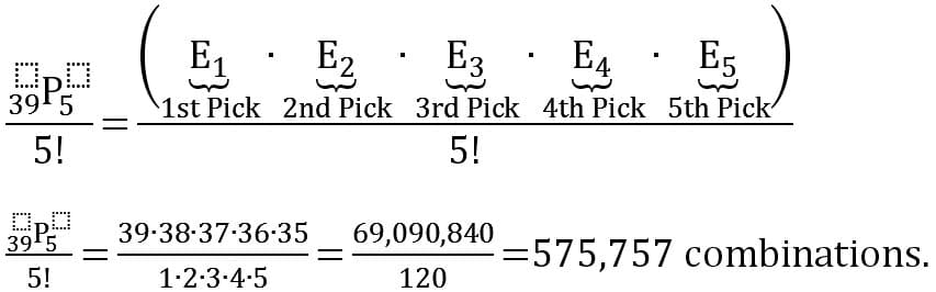
For the first pick, E₁=39, since there are 39 choices. Since no numbers can be repeated, E₂=38. Since each pick leaves one less option, E₃=37, E₄=36 and E₅=35. This gives the total number of permutations as E=(39)(38)(37)(36)(35)=69,090,840 permutations.

There are just over 69 million ways to select a sequence of 5 numbers from the set of numbers 1 to 39, but we want combinations. This means that we don’t care about the ordering of the 5 numbers, only about the set we get. Notice that we could have picked the same numbers in a different order. For example, the formula above treats the sequence of 5 numbers, 9, 11, 18, 25, and 31, as different from the sequence of 5 numbers 11, 25, 9, 31, 18, despite the fact that they both give the same collection of numbers. From this observation, I would say to my students: Didn’t we find a way to account for distinguishable permutations, that is, different orderings, already? I would also ask, “How many repeats of each number set are within the 69,090,840 permutations?”

I want my students to see the connection between, r, the number of elements being chosen, and the number of repetitions for each set of r numbers. Taking 5!=120, gives the number of times each distinct set of 5 is counted in the 69,090,840 permutations. Thus, for each combination, there are 120 different permutations that are accounted for in the 69,090,840 permutations. Thus, to find the number of distinct combinations, we would divide by 5!

This is one of multiple examples I would show students before generalizing the formula for combinations. I will take the time to show how to break down the problems into smaller pieces that utilize prior concepts rather than just giving the formula. By understanding the problem, students would be better equipped to identify whether a question was seeking permutations or combinations. Knowing what type of problem would enable them to select the correct formula to solve the problem.

Combinations and the Binomial Theorem

Textbooks often point out the fact that the binomial coefficients found in Pascal’s Triangle also tell us the number of combinations when choosing r objects from n items. Often, students are told to count to the nth row of the triangle and then find the rth entry. To convince my students of this fact, I would have students group for 0≤r≤n when n=1, 2, 3, 4 and 5.  The definition 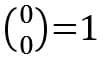would be given to students. I would have to introduce the concept of the empty set, ϕ, counting as 1 set. I expect this to be a difficult concept for students to comprehend, even at the precalculus level.

To explain this concept, I would ask my students, “How many ways can we take 0 items from a group of n?” It seems odd that the result is 1, but if we were to select 0 items, we would have 0 items afterwards, thus there is 1 way to have 0.

By having students list out and count the number of sets will make the connection between the number on Pascal’s Triangle and ^⧠_nC^⧠_r more apparent, because they will be writing out the actual set combinations for each situation.

For, n=1, {A}.

For, n=2, {A, B}.

For, n=3, {A, B, C}.

I will have my students construct similar tables for the cases where n=4 and n=5. Writing out the combinations and counting the ways for selecting r elements from a group of n for 0≤r≤n gives a more concrete way to connect the binomial theorem coefficients with ^⧠_nC^⧠_r. This exercise emphasizes the connection between the number of subsets with the coefficients of the binomial theorem.

An additional exercise I would introduce to students is to demonstrate how to produce subsequent rows of Pascal’s Triangle using the recursion formula 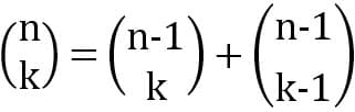. For example, .

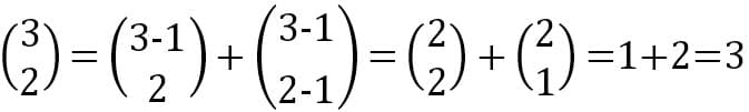I will have my students compute more examples to show the recursion formula works numerically. For more advanced students, I would challenge my students use mathematical induction to confirm the recursion for Pascal’s Triangle by showing using the formula for .