Background
Far too often my students become intimidated by, shy away from and struggle with the sight of fractions in any form. They have trouble with decimals and knowing place values, especially within word problem scenarios. Herb Gross 3 describes this as "math phobia": my students have such a fear of math that they deny themselves the upward mobility that would come with success in this subject area. In this unit, I am seeking ways to make the content of mathematics appealing to students through practical applications of math concepts.
Students need to be guided to do math, and it should be presented in a non-threatening way that is easy to internalize. Perhaps it would be helpful for students to view learning math as a game in which they are being exposed to math concepts using video lectures, PowerPoint presentations, animation and even something as simple as user friendly text that they can easily read and digest through graphic organizers and other means of organizing content knowledge. The seminar discussions and readings from Roger Howe's seminar "Place Value, Fractions, and Algebra: Improving Content Learning through the Practice Standards" brought forth the misconceptions and challenges students face when working with these mathematics topics in math courses at all levels. While many conversations occurred throughout the two weeks of the seminar, the topic discussed most was how to teach fractions in a way that students will understand. I automatically connected this with the difficulty my students have with recognizing slopes of linear functions, or rate of change from one point on a straight line to another, as a fraction.
Many of the fraction skills that are reviewed in the first year of high school mathematics, typically an Algebra 1 course, should have been first learned in third through the fifth grade and then solidified in the sixth through eighth grade math courses, so that high school students would be confident in working with fractions. However, this is often not the case with my students. My hope for this curriculum unit is that students accept the challenge of identifying rate of change as a fraction and apply this knowledge to linear functions in word problem scenarios. I want students to delve into real life scenarios with confidence and ease and to recognize that the process needed to arrive at a solution is just as important as the final answer.
The completion of Modules 1, 2 and 3 of the MVP curriculum will precede this curriculum unit. These modules will require students to define quantities and interpret expressions, to use units to describe variables, to understand problems, and to explain each step in a process to solve an equation. These modules will also include work with ratios, unit fractions, fractions with fixed denominators and fractions with different denominators. Students will have used the number line model to interpret unit fractions and general fractions, and how to use fractions to measure distance from zero to a given point on the number line. Students will have seen a coordinate plane and will understand how to place whole numbers, integers and fractions on the x-axis and y-axis. All this content knowledge is needed for the activities of this curriculum unit.
Fractions
Throughout the Common Core State Standards for Mathematics (CCSS-M) courses from elementary and middle school, students will have been exposed to the process of understanding the practical application of fractions in their everyday lives to provide a context for processing simple word problem scenarios. Upon entering the CCIM-I course, students should have a basic understanding of multiple representations of fractions and ratio. This curriculum unit will relate this prior knowledge to rate of change in everyday life scenarios.
I will expect my students to start this unit with the understanding that, in everyday life, all numbers come with units attached. In other words, all numbers can be considered adjectives that relate to a noun 4. A fundamental convention of arithmetic is, that when we add numbers, they all must refer to the same unit. An example would be to use coins, such as nickels, dimes, and quarters. Consider that 3 dimes and 4 nickels are equivalent to 2 quarters. However, we would never write this as 3 + 4 = 2. Instead, we would refer each coin to its value in a common unit, for example cents: 5 cents per nickel, 10 cents per dime and 25 cents per quarter. By using coins as the noun, their unit value and the number of coins becomes the adjectives: 3 coins worth 10 cents each for a total of 30 cents combined with 4 coins worth 5 cents each for total of 20 cents is equivalent to 2 coins worth 25 cents each for a total of 50 cents. This unit consciousness will be extended in class discussions whose goal is to identify the more complicated units of quantities being used for ratios as unit fractions and general fractions.
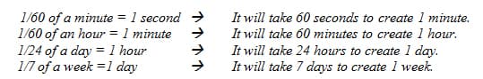
Ratios in fraction form express parts of a certain quantity (numerator) in comparison to a specific unit (denominator). This is illustrated in unit fractions and general fractions. The CCSS-M approach to fractions is based on unit fractions. The unit fraction 1/d of some unit is a quantity such that it takes d copies of 1/d to make the original unit. Unit fractions are considered as 1/d pieces of a whole unit. General fractions in the form of n/d are multiples of unit fractions: n copies of 1/d produces n/d. For example, we use unit fractions in our system for measuring time:
Although it is not part of the CCSS-M definition of fractions, it is important in general, and especially for my curriculum unit, that students understand that a fraction also represents the result of a division. Thus, ¾ is defined as 3 pieces of size ¼ each, but it also is equal to the result of dividing 3 into 4 equal pieces. Realizing this equivalence will be necessary for my students to understand rates of change expressed as fractions.
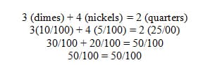
The notion of units of measurement should be addressed within the ratios produced by fractions. Students will need to interpret the relationship between values in the numerator and denominator of a fraction: the numerator will be dependent upon the unit being used in the denominator. This establishes the independent and dependent relationship between the units being used to create the ratio. Students will identify these units to interpret the meaning of a ratio with relation to the scenario or context with which the ratio is being used. Consider the coins example in which 3 dimes and 4 nickels are equivalent to 2 quarters. The value of all three coins is a multiple of 1/00 of a whole dollar: each dime is 10 times 1/100 or 10/100 of a dollar, each nickel is 5 times 1/100 or 5/100 of a dollar and each quarter is 25 times 1/100 or 25/100 of a dollar. When illustrating the equivalence of these values using the same units we see that:
The unit conversion relating all coin values to a dollar in the form of a ratio helps to compare the resulting fractions using the same unit of measurement. This understanding of ratios will translate into understanding how constant rates of change in the form of a ratio with specific units relate to slope.
Slope and Straight Lines
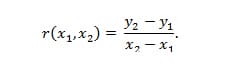
Given two points P 1 = (x 1, y 1) and P 2 = (x 2, y 2) in the Cartesian coordinate plane, the slope between P 1 and P 2 is the quotient or ratio
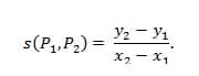
Since y 2 – y 1 is the vertical change, or "rise" in carpenter's terminology, in going from P 1 to P 2, and x 2 – x 1 is the horizontal change, or "run", slope is also referred to as "rise over run", or rise divided by run. Sometimes, the difference or change in y-values in going from P 1 to P 2 is written as Δy = y 2-y 1, and in similar fashion, the difference or change in the x-values is written as Δx = x 2-x 1. The slope between P 1 and P 2 can then be represented with the notation Δy/Δx. We will use this notation for this curriculum unit.
I want my students to understand that slope is exactly the right quantity to look at when dealing with straight lines in the coordinate plane. The intuitive idea of a straight line is precisely and elegantly captured by the condition of constant slope. When a set of points is given, whether or not they are in numerical order with respect to the independent (x) value of the point, and the slope between any two of the given points is the same as between any other two of the points, the whole collection of given points will all lie on a single straight line. While it is often helpful to list coordinate points in numerical order, it is not necessary when determining the slope between the points. The set of given points can be in any order and any two points can be used to find the slope, so long as the resulting slope is exactly the same every time for any pair in that particular set of points. The straight line passing through all of the given points can then be described by a simple equation. If P 1 = (x 1, y 1) is a selected one of the points, and P= (x, y) is any other point in on the line, and if m is the slope, then if we multiply both sides of the equation

by x – x 1, we get the equation
y-y 1=m(x-x 1 ).
By adding y 1 to both sides and expanding the product on the right hand side, this equation can be rewritten as
y=mx+(y 1-mx 1 )= mx+b.
We will interpret the constant b = y 1 – mx 1 later on. This underlines the fact that there is a constant linear relationship between the dependent (y) and independent (x) values of points on a straight line. I will have my students work out many numerical examples of this remarkable characterization of straight lines, some purely numerical, and others arising in real-world scenarios, until they become convinced of its truth.
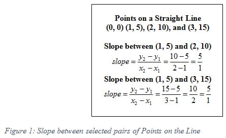
The slope (m) between any two coordinate points from the same straight line will always be exactly the same. This can be verified by choosing a set of points from a straight line, then calculating and comparing the resulting slopes from any two points on the straight line (Figure 1). To calculate the slope, determine the change in y-values (Δy) in the numerator in relation to the change in x-values (Δx) in the denominator:
m = Δy / Δx = (y 2-y 1) / (x 2-x 1).
I will have my students check the following key fact in many cases, with the hope that they will make the generalization: Given any three points, P 1, P 2, and P 3, if the slopes between P 1 and P 2 and between P 2 and P 3 are the same, then the slope between P 1 and P 3 is also equal to the common value of the first two slopes. This is illustrated in Figure 1.
Related quantities
There are many situations in which two quantities are related in some way. For example, if someone has a bank account at a bank and makes regular deposits, the amount of money in the account will grow with time. Or if someone has some money, and uses it to buy things, the amount they have left will depend on the purchases. If what is needed is multiple copies of a single product, the amount left will depend on the number of copies bought. Or if someone has an exercise program that includes running, and runs a fixed amount each day, the total distance run will depend on the number of days the program has been followed.
Usually in these situations, we think of one quantity as determining the situation, and the other as depending on the first. In first and third examples above, time runs along (whatever we do), and the quantity we are interested in (bank account value, or distance run), depends on the time. In the middle example, we decide how many copies of a given product we need, and then the money we have to spend, and the money we have left, depends on the number of copies. We use the terminology independent variable to refer to the variable that controls the situation, and dependent variable to refer to the other quantity, whose value is determined by the value of the independent variable.
Table of Values
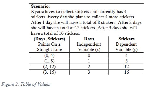
If we have a pair of related quantities, we can describe the relationship by creating a table of values. The table of values serves as a means to organize and identify the relationship between dependent (y) and independent (x) variables in a sequential order. Since it is frequent practice for the x values chosen to make a table of values are consecutive whole numbers, it is common practice to set up a table of values by using a two column table and placing the value of the independent (x) variables in numerical order in the first column and then listing the corresponding values of the dependent (y) variable in the second column. In Figure 2 a table of values is used to identify the relationship between two variables from a specific scenario. In the situations we will study, which involve only linear functions, the y-values will also be in numerical order of increasing or decreasing value in the table. Note that the table of values will eventually be used to graph the coordinate points and develop a linear equation, so it will be helpful for students to become familiar with identifying the value of y when x is zero in their table of values. Students will later identify this coordinate point as the y-intercept.
Rate of change
When two quantities are related, one is often interested in knowing how much a change in the independent variable affects the dependent variable. It turns out to be useful to look, not just at the change in the dependent variable, but at the rate of change. This is defined as follows: Given two values, x 1 and x 2, of the independent variable, and two corresponding values, y 1 and y 2, of the dependent variable, the rate of change of y between x = x 1 and x = x 2 is the ratio or quotient 777
It might not be obvious to my students why we should look at the rate of change. The formula may look complicated. I want to get them to understand that the rate of change is the key to understanding the wide variety of scenarios that we study. The remarkable thing about these scenarios is that the rate of change turns out to be constant, and completely independent of the two values of x that are chosen. Thus, in our scenarios, if we know the rate of change, and the value of y for a single value of x, we can compute the value of y for any value of x. The entire relationship can be encoded with just two numbers!
Graphing a relationship
Even though the variables in a relationship (money, time, number of items purchased) may have no geometric significance, once we have recorded the relationship in a table of values, it is tempting to graph the pairs of values as points in a coordinate plane. I want my students to understand that, when we do this, we get a relationship between geometry and numerics: the rate of change that was a key to understanding linear relationsh ips turns into the slope between points, and the graph of a relationship with constant rate of change is a straight line!
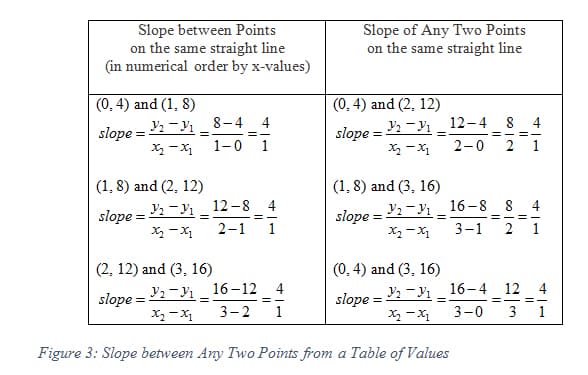
When the structure of a table of values is set so that the rate of change between any two values of the independent variable is the same, then, when the table is graphed, this relationship will be seen as the slope of a straight line through any two points chosen from the table. This can be seen in Figure 3 where any two points are chosen from the table of values and when the slope is calculated, the result is exactly the same each time. The recognition of this slope in relation to the difference in dependent (y) and independent (x) variables will translate into plotting points from the table, in any order, on a coordinate plane to create a visual representation of the linear relationship between two variables.
The constant rate of change of 4/1 in Figure 3 indicates that when the coordinate points are placed on a coordinate plane, beginning with the coordinate point (0, 4) the next point will be four units up and one unit to the right from the beginning point. In essence, the resulting slope that is determined by finding the "rise over run" of the dependent (y) and independent (x) variables indicates that when we want to determine the value of coordinate points on a straight line, begin with one coordinate point, usually the first point from a table of values in numerical order, and use the slope to move the specified units to the next coordinate point. Continuing this pattern will result in the creation of a graph of a straight line.
Graph of a Linear Relationship
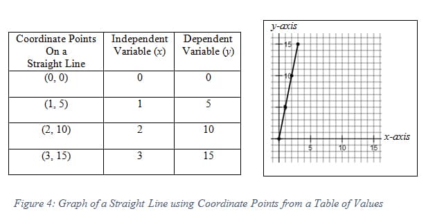
The coordinate plane consists of all the possible values of the independent (x) variable along the horizontal, or x-axis and all of the possible values of the dependent (y) variable along the vertical, or y-axis. The units labeled along each axis represents the value of the variables. The points from a table of values are called coordinate points in the form (x, y). The values of each variable within the coordinate point determines the location of that point within the plane. For example, we see in Figure 4 that when a table of values is created for the coordinate points (0, 0), (1, 5), (2, 10), and (3, 15), the independent (x) values are in order from least to greatest and all dependent (y) values are adjacent to the corresponding x-values. All four points are then drawn onto the coordinate plane and connected in numerical order to create a straight line.
Linear Functions in Slope-Intercept Form
A straight line can also be described as the graph of a linear function. There is a constant slope between any two coordinate points, and every independent (x) value has exactly one dependent (y) value related to it. The slope between these coordinate points can be verified by determining the rate of change in a table of values. It is important to note that the previous examples of linear functions have all included an x-value of zero as the first coordinate point in the table of values and on the graph. This is intentional since that specific coordinate point is the location where the graph of the straight line intersects or crosses the y-axis. This coordinate point, known as the y-intercept, is the beginning point of the graph of a linear function and the slope is then used to move at a constant rate of change from that beginning point to all other coordinate points to create the graph of a straight line, thus forming a graphical representation of a linear function.
The coordinate points (x, y) become values that can be substituted, or replaced, for the x and y variables in the linear equation to validate that the given coordinate points will appear as points on the graph of the linear function. This validation also proves that the given coordinate points are now solutions to the linear equation representing the linear function. Consider the coordinate points (0, 6), (1, 13), (2, 20), and (3, 27) which can be organized into a table of values and then graphed in a coordinate plane to create a straight line. The slope between any two points from this set of given coordinate points would be 7/1, indicating that as the x-values increase by 1 unit, the y-values increase by 7 units. To illustrate the relationship of taking any coordinate point (x, y) and moving with the slope (rise/run) to determine the continuous coordinate points in a linear function, we use the notation (x, y) —> (x + run, y + rise), where (x + run, y + rise) represents the next numerical coordinate point in the sequence of coordinate points for the linear function. For example, since we already know the slope of this specific linear function is 7/1, by following the notation we see a relationship developing between continuous coordinate points, using the slope between two points and beginning with the y-intercept:
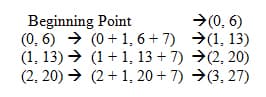
The result of using this notation has produced continuous coordinate points that can now be graphed on a coordinate plane in a straight line to produce a linear function.
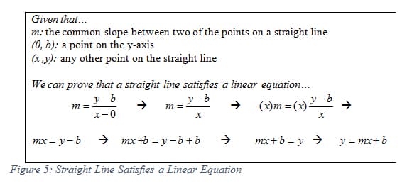
Slope-Intercept Form of a Linear Equation
The relationship between the slope, y-intercept, and coordinate points to create the graph of the linear function can be represented in the form of a linear equation y=mx+b, known as the slope-intercept form (Figure 5). The slope (m) is identified as the rate of change between any two coordinate points (x, y). The y-intercept (b) is a specific point of interest where the graph begins. The y-intercept will be identified as the coordinate point (0, b) to denote that the x-value is always equal to zero, and the y-value will indicate the y-intercept, or the location where the linear function will intersect with the y-axis. Returning to the previous example of a linear function whose slope is 7/1 and y-intercept is (0, 6), these values can be used to create the slope-intercept form of this linear function by substituting 7/1 (or just 7) for the slope (m) and 6 for the y-intercept (b): y = 7x + 6. This linear function is telling us that the graph of this function would begin at (0, 6) and move or rise 7 units up for each run of 1 unit to the right, so when x changes from 0 to 1, we would arrive at the point on the graph (1, 13). From this new point, the slope would continue to rise 7 units for each run of 1 unit to arrive at other points.
Coordinate Points as Solutions to Linear Equations
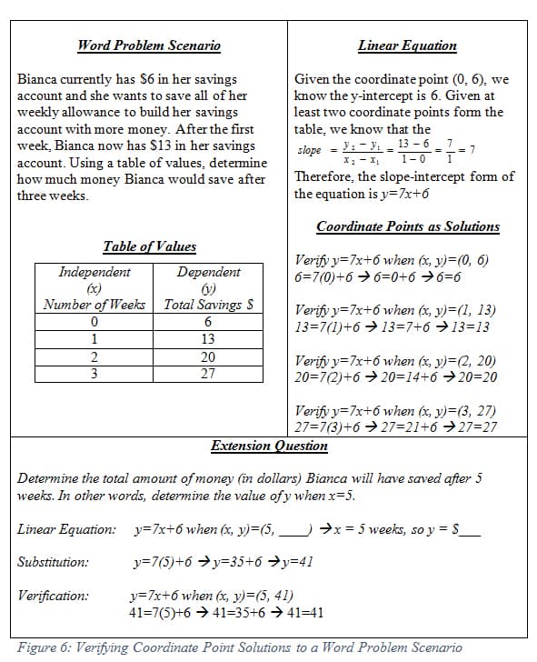
Linear equations can be created and used to understand, interpret and determine solutions to simple and complex word problem scenarios involving two variables related by a linear function. The process to create these linear equations is to identify the dependent (y) and independent (x) variables from the word problem scenario and create a table of values to organize the relationship between the variables. By computing the rate of change for each pair of adjacent values of the independent variable, students can recognize whether the relationship is linear by checking whether all the computed rates of change are the same. Using the slope and y-intercept derived from a table of values or a graph, a linear equation can be created to represent the linear relationship between the variables. Once this linear equation has been created, all the coordinate points from the table of values can be verified as being solutions to the equation by substituting the coordinate points into the linear equation, resulting in a true statement. There is a sequence of steps to create a linear equation from a word problem scenario and prove that coordinate points are solutions to the linear equation (Figure 6). Although when graphed, the relationship appears to have turned into pure geometry, it is important to remember its real world origins. To make sure that my students stay in touch with the real world meaning, I will ask them always to label the x- and y- axes to show the quantities they represent, including units.
An extension to the word problem scenario in Figure 6 may require an extension of the table of values and the use of the linear equation to determine another solution. The extension question shows how the linear equation could be used to identify and verify the solution to prove its relevance to the extension question. The ability to determine the solution to the extension question will assess student understanding of the relationship between the two variables, slope and y-intercept.
Comments: