From Arithmetic to Algebra: Variables, Word Problems, Fractions and the Rules

Quadratic Sequences

Quadratic sequences are characterized by having a constant second difference. This is often stated as fact in textbooks. In the curriculum my school uses, there are no explanations as to why a second constant difference implies we have a quadratic equation. By searching through multiple high school curriculum resources, I have found that the second common difference is usually presented through examples, and students are told that if they find a constant second difference, they know they have a quadratic sequence. Though students are expected to write the equation of a quadratic sequence, many exercises rely on knowing key features of quadratics, such as the vertex or both intercepts.

Al Cuoco outlines one method to find the equation of a quadratic function in Mathematical Connections.⁴ The procedures involve taking a quadratic sequence and creating a table that includes an analysis of the first difference, ∆, and the second difference, ∆∆ which is found by taking the differences of the first differences. Using this structure as a starting point, and using the skill of creating a first difference table for arithmetic sequences, an equation can be constructed for any quadratic sequence.

Quadratics are studied in Integrated Math 2 and subsequent math courses. In Math 1, students will have practiced using both the sequence notation, a_n, and the function notation, f(n), to represent sequences. For the purpose of the following example and its place in the mathematics curriculum currently used in my school, function notation will be used. The following exercises will show that a unique quadratic equation can be written for a given sequence with constant second differences. In particular, the exercises will demonstrate:

1. A Quadratic function implies constant second difference.
2. How to reconstruct a quadratic function from its second difference.
3. A constant second difference implies we have a quadratic. This is meant to be an algebraic exploration of quadratic functions that will assist students with understanding how to analyze quadratic sequences and make generalizations.

The General Quadratic Sequence

There are three ways of connecting a quadratic sequence with its first and second difference sequences:

i) You can compute the coefficients d and e of the first difference sequence dn + e, and the value d of the second difference sequence, in terms of the coefficients ax²+bx+c of the orginal sequence, and solve for a, b, c in terms of d and e, and the first value a+b+c of the sequence.

ii) You can sum the first n (or n-1) terms of the first difference sequence (and add the first value of the sequence to that sum). This can be done in two ways: iia) geometrically or iib) by formal algebraic computation.

In this section, approach (i) will be used to express a quadratic function in terms of its first and second differences. The next section will show by example how both methods (i) and (iia) can produce the same quadratic equation. Cuoco utilizes formal algebraic computation in Mathematical Connections, and I will not use method (iib) as it requires use of combinatorics, which is beyond the scope of the courses for which this unit is intended.

General Quadratic Equation

The following exercise outlines one process that can be used to analyze a sequence that is quadratic in order to write an equation in the form ax^2 +bx+c. Though this example uses the general quadratic equation as a starting point, I would consider starting by examining quadratic number sequences, such as 1, 4, 9, 16, 25, … before showing this process to my students. 

We begin by considering the standard form of a quadratic equation, f(x)=ax^2 +bx+c, where a,b, and c are real numbers with a≠0.

First, we evaluate the function for the integers from 1 to n.

f(x)=ax² +bx+c

f(1)=a(1)² +b(1)+c=a+b+c

f(2)=a(2)² +b(2)+c=4a+2b+c

f(3)=a(3)² +b(3)+c=9a+3b+c

f(4)=a(4)² +b(4)+c=16a+4b+c

f(5)=a(5)² +b(5)+c=25a+5b+c

…

f(n-1)=a(n-1)² +b(n-1)+c=a(n-1)² +b(n-1)+c

f(n)=a(n)² +b(n)+c=an² +bn+c

As a sequence: (a+b+c),(4a+2b+c),(9a+3b+c),…,(an² +bn+c) 

As a table:

The next step is to take the first difference, ∆_x =f(x+1)-f(x). Note that the first differences in this example use function notation, whereas the linear example above used the sequence notation Δ_n =a_n+1 -a_n.

For x=1,∆₁ =f(2)-f(1)

∆₁ =(4a+2b+c)-(a+b+c)=3a+b

For x=2,∆₂ =f(3)-f(2)

∆₂ =(9a+3b+c)-(4a+2b+c)=5a+b

…

For x=n-1,∆_n-1 =f(n)-f(n-1)

∆_n-1 =f(n)-f(n-1)

=(an² +bn+c)-(a(n-1)² +b(n-1)+c)

=an² +bn+c-a(n-1)² -b(n-1)-c

=a(n² -(n-1)²)+b(n-(n-1))+(c-c)

=a(n² -(n² -2n+1))+b(n-n+1))+(c-c)

=a(2n-1)+b(1))+(0)

=(2n-1)a+b.

Adding a column to our table, we record the first differences.

All of the steps up to this point were used to determine if a sequence is arithmetic. We notice that the first difference is not constant. I will ask my students to look at the first differences carefully, and I hope that they will be sufficiently comfortable with arithmetic sequences to recognize that this difference sequence is arithmetic.

Writing the first difference sequence, we have:

3a+b, 5a+b, 7a+b, 9a+b, …, a(2n-3)+b, a(2n-1)+b.

Since we know how to analyze an arithmetic sequence, we use the same process to analyze the first differences. We will accomplish this by taking the second difference, ∆∆_x =∆_x+1 -∆_x.

For x=1, we have,

∆∆₁ =(5a+b)-(3a+b)=5a+b-3a-b

=5a-3a+b-b

=2a.

For x=2,

∆∆₂ =(7a+b)-(5a+b)=7a+b-5a-b

=7a-5a+b-b

=2a.

And so on…

Taking x=n-2

∆∆_n-2 =(2n-1)a+b-((2n-3)a+b)=2an-a+b-2an+3a-b

=2an-2an-a+3a+b-b

=(2an-2an)+(-a+3a)+(b-b)

=(0)+(2a)+(0)

=2a.

Expanding our table by adding a fourth column, the table is a second difference table for the quadratic.

Observe that ∆∆_x =2a for 1≤x≤n.The second difference table shows that a general quadratic, f(x)=ax² +bx+c has a constant second difference. This demonstrates condition (1). 

Next, we want to show that a quadratic can be reconstructed from the second difference. Though this procedure is not shown in the math textbook we use, I definitely plan to show this to my pre-calculus students, and to my Math 1 students if there is additional time, because it connects the constant second difference and first difference to the equation of a quadratic. To accomplish this feat, we use the general theorem that a sequence is determined by its first term and its difference sequence. Applying this twice, we will get our quadratic.  

Using the information in the second difference table, notice that the second difference is constant. We can express this relationship in the equation, 2a=∆∆. Solving for a, we have

2a=∆∆

2a/2 = ∆∆/2

a= ∆∆/2.

The result shows us that for a quadratic sequence, the coefficient of the x² term is equal to half the second common difference. I would point out to my students that the second difference of a quadratic effects the vertical stretch of a quadratic because it is twice the leading coefficient.

Since we can find the value for a, we need to find the b and c values. The method is to remove the quadratic component of the sequence by subtracting the ax² from each term. Let g(x)=f(x)-ax². This gives us

g(x)=f(x)-ax² =(ax² +bx+c)-ax² =bx+c.

By doing so, we have a linear equation g(x)=bx+c. Evaluating this expression for values 1≤x≤n, we can make a new table, which we will analyze.

From the table above, we will attempt to analyze the values obtained by finding ∆_x^', the first difference of g(x).

Computing the first difference shows that ∆_x^'=b for all of the first differences. Thus, the coefficient of the x term in the quadratic is equal to the first difference of f(x)-ax². Since the first difference is constant, we showed that f(x)-ax² is linear. At this point, I would expect my students to notice that they have a linear sequence and would be able to write the general expression c+∆_x^'.

This shows that f(x)-ax² =c+∆'x, which we can then solve for c, by subtracting ∆'x from both sides of the equation. Substituting b for ∆' and ax² +bx+c for f(x), we have

c=f(x)-ax² -∆^' x

=ax² +bx+c-ax² -bx

=c, for all x.

I would point out that a quadratic equation in the form f(x)=ax² +bx+c can be written for a sequence with constant second common difference ∆∆ if we follow the three steps:

Step 1: To find a, take a= ∆∆/2.

Step 2: b is the the first common difference, ∆', of the sequence formed by subtracting (∆∆/2)x² from each term in the original sequence.

Step 3: We can find the constant value c, by subtracting ((∆∆/2)x² +∆^'x) from any term in

the original sequence.

Though the computations can be tedious, the process is an extension of the difference tables used to analyze arithmetic/linear sequences. One valuable outcome in going through this process is to emphasize the fact that quadratic functions are characterized as having a second common difference, which lays the foundation for calculus and the study of rates of change and derivatives.  In calculus, one could characterize quadratic functions as those functions with constant second derivative. Another outcome is that there is a way to write an explicit equation for quadratic sequences, though it does require some work.

Example of a Quadratic Sequence

The Handshake Problem: There is a party. Each person at the party shakes the hand of every other person in the party. People are unable to shake hands with themselves, and you are not counting multiple handshakes with the same person. Starting with two people, create a sequence with five terms to show the relationship between the number of people at the party and the number of handshakes. Then write a function to determine the number of handshakes if there are n people at the party.

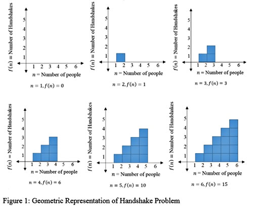
To start this problem, one approach is to make a table with columns indicated the number of people at the party and number of handshakes. With two people, persons A and B, at the party, there is only one handshake possible. If a third person, C, arrives, there will be two additional handshakes as C must shake hands with A and B, for a cumulative total of 3 handshakes. If a fourth person, D, arrives, the only new handshakes are between D and each of the three other guests, for a total of 6. If a fifth person E arrives, there are four more handshakes for a total of 10. Continuing the trend, with each new arrival, the person must shake hands with those already present. So when a sixth person arrives, there are five more handshakes for a total of 15 and so on.

Note that this constructing of the handshake function uses an argument based on what its first difference sequence must be, and adding the differences. This argument shows that the difference sequence is linear which will allow us to conclude that the original sequence is quadratic because a linear first differences implies constant second differences.

As a starting point, we can compute the first difference using ∆_n.

We notice that the first differences are not constant, but appear linear. This sequence could be quadratic, so we should check to see if there if the second difference is constant. Computing ∆∆_n, we extend our table and observe that the second common difference is constant. Therefore, we will be able to write a quadratic equation in the form an²+bn+c for the handshake problem.

With ∆∆_n =1, we find a by taking a = ∆∆_n/2 = ½.

To find the value of b and c, we take our original values for the number of handshakes and subtract (∆∆_n/2) n² = ½n² from each term.

From these values, we will now compute the first differences, ∆^'_n.

Since the first difference ∆^'_n is constant, we know from the explanation above that b=∆^'_n=-½. We then can find c using the formula c=f(n)-( ∆∆_n/2)n² -∆^'_n. For n=1, we have

We can rewrite this equation in the form f(n)= ½(n)(n-1).

This is one way that we can find an algebraic representation for the handshake problem, based on the structure outlined in the prior example.

Geometric Representation of Handshake Problem

An alternative approach to write an equation that models the handshake problem is represent it geometrically using a graph. See Figure 1.

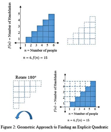
Examining the shape of the geometric function, observe that if we were to copy the exact figure, rotate the figure 180°, then we could combine the rotated figure and the original one to make a rectangle.

Observe the resulting rectangle’s horizontal and vertical lengths and their relation to n. See Figure 3. The horizontal length is equal to n units, while the vertical length is n-1 units. Thus, its area is given by n(n-1). The total area of the rectangle represents double the number of handshakes.

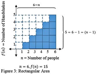
To get the area of the shaded region, we can take half of the area of the rectangle. The resulting equation can be written as f(n)= ½ (n)(n-1), which is equivalent to our equation found using the first term, first difference and second difference sequences. From the handshake problem example, both a computational algebraic approach and a geometric visual representation produced equivalent equations that modeled the situation. Interpreting problems in multiple representations will provide opportunities for students to see the connections between the first and second differences and quadratic equations.

Throughout this unit, difference sequences will be used to analyze original sequences. Noticing key features will help students to identify arithmetic, geometric and quadratic sequences. Though they are the three special cases that are given most of the attention at the high school level, there are many more types of sequences that do not receive as much attention, but can be explored by analyzing difference sequences. Starting in the Integrated Math 1 classes, students will develop the tools that can be applied to linear, exponential, and quadratic functions. At the Math Analysis level, repeated applications of the general theorem for difference sequences is a tool to analyze polynomial functions. By taking time to understand the roles of the differences, students will see an alternative approach to write algebraic equations that model numerical patterns.